Introduction to Neural Networks using TensorFlow
It is prudent to use Neural Networks for complex problems such as image processing. Neural nets belong to a class of algorithms called representation learning algorithms. These algorithms break down complex problems into simpler form so that they become understandable (or "representable"). Think of it as chewing food before you gulp. This would be harder for traditional (non-representation learning) algorithms. When you have appropriate type of neural network to solve the problem. Each problem has its own twists. So the data decides the way you solve the problem. For example, if the problem is of sequence generation, recurrent neural networks are more suitable. Whereas, if it is image related problem, you would probably be better of taking convolutional neural networks for a change. Last but not the least, hardware requirements are essential for running a deep neural network model. Neural nets were "discovered" long ago, but they are shining in the recent years for the main reason that computational resources are better and more powerful. If you want to solve a real life problem with these networks, get ready to buy some high-end hardware!General way to solve problems with Neural Networks
TO DO list of how to approach a Neural Network problem. Check if it is a problem where Neural Network gives you uplift over traditional algorithms (refer to the checklist in the section above) Do a survey of which Neural Network architecture is most suitable for the required problem Define Neural Network architecture through which ever language / library you choose. Convert data to right format and divide it in batches Pre-process the data according to your needs Augment Data to increase size and make better trained models Feed batches to Neural Network Train and monitor changes in training and validation data sets Test your model, and save it for future use For this article, I will be focusing on image data. So let us understand that first before we delve into TensorFlow.Understanding Image data and popular libraries to solve it
Images are mostly arranged as 3-D arrays, with the dimensions referring to height, width and color channel. For example, if you take a screenshot of your PC at this moment, it would be first convert into a 3-D array and then compress it ‘.jpeg' or ‘.png' file formats. While these images are pretty easy to understand to a human, a computer has a hard time to understand them. This phenomenon is called "Semantic gap". Our brain can look at the image and understand the complete picture in a few seconds. On the other hand, computer sees image as just an array of numbers. So the problem is how to we explain this image to the machine? In early days, people tried to break down the image into "understandable" format for the machine like a "template". For example, a face always has a specific structure which is somewhat preserved in every human, such as the position of eyes, nose or the shape of our face. But this method would be tedious, because when the number of objects to recognise would increase, the "templates" would not hold. Fast forward to 2012, a deep neural network architecture won the ImageNet challenge, a prestigious challenge to recognise objects from natural scenes. It continued to reign its sovereignty in all the upcoming ImageNet challenges, thus proving the usefulness to solve image problems. So which library / language do people normally use to solve image recognition problems? One recent survey I did that most of the popular deep learning libraries have interface for Python, followed by Lua, Java and Matlab. The most popular libraries, to name a few, are: Caffe DeepLearning4j TensorFlow Theano Torch Now, that you understand how an image is stored and which are the common libraries used, let us look at what TensorFlow has to offer.What is TensorFlow?
Lets start with the official definition,"TensorFlow is an open source software library for numerical computation using dataflow graphs. Nodes in the graph represents mathematical operations, while graph edges represent multi-dimensional data arrays (aka tensors) communicated between them. The flexible architecture allows you to deploy computation to one or more CPUs or GPUs in a desktop, server, or mobile device with a single API."

 If that sounds a bit scary – don't worry.
Here is my simple definition – look at TensorFlow as nothing but numpy with a twist.
If you have worked on numpy before, understanding TensorFlow will be a piece of cake! A major difference between numpy and TensorFlow is that TensorFlow follows a lazy programming paradigm.
It first builds a graph of all the operation to be done, and then when a "session" is called, it "runs" the graph.
It's built to be scalable, by changing internal data representation to tensors (aka multi-dimensional arrays).
Building a computational graph can be considered as the main ingredient of TensorFlow.
To know more about mathematical constitution of a computational graph, read this article.
It's easy to classify TensorFlow as a neural network library, but it's not just that.
Yes, it was designed to be a powerful neural network library.
But it has the power to do much more than that.
You can build other machine learning algorithms on it such as decision trees or k-Nearest Neighbors.
You can literally do everything you normally would do in numpy! It's aptly called "numpy on steroids"
The advantages of using TensorFlow are:
It has an intuitive construct, because as the name suggests it has "flow of tensors".
You can easily visualize each and every part of the graph.
Easily train on cpu/gpu for distributed computing
Platform flexibility.
You can run the models wherever you want, whether it is on mobile, server or PC.
If that sounds a bit scary – don't worry.
Here is my simple definition – look at TensorFlow as nothing but numpy with a twist.
If you have worked on numpy before, understanding TensorFlow will be a piece of cake! A major difference between numpy and TensorFlow is that TensorFlow follows a lazy programming paradigm.
It first builds a graph of all the operation to be done, and then when a "session" is called, it "runs" the graph.
It's built to be scalable, by changing internal data representation to tensors (aka multi-dimensional arrays).
Building a computational graph can be considered as the main ingredient of TensorFlow.
To know more about mathematical constitution of a computational graph, read this article.
It's easy to classify TensorFlow as a neural network library, but it's not just that.
Yes, it was designed to be a powerful neural network library.
But it has the power to do much more than that.
You can build other machine learning algorithms on it such as decision trees or k-Nearest Neighbors.
You can literally do everything you normally would do in numpy! It's aptly called "numpy on steroids"
The advantages of using TensorFlow are:
It has an intuitive construct, because as the name suggests it has "flow of tensors".
You can easily visualize each and every part of the graph.
Easily train on cpu/gpu for distributed computing
Platform flexibility.
You can run the models wherever you want, whether it is on mobile, server or PC.
A typical "flow" of TensorFlow
Every library has its own "implementation details", i.e. a way to write which follows its coding paradigm. For example, when implementing scikit-learn, you first create object of the desired algorithm, then build a model on train and get predictions on test set, something like this: # define hyperparamters of ML algorithm clf = svm.SVC(gamma=0.001, C=100.) # train clf.fit(X, y) # test clf.predict(X_test) As I said earlier, TensorFlow follows a lazy approach. The usual workflow of running a program in TensorFlow is as follows: Build a computational graph, this can be any mathematical operation TensorFlow supports. Initialize variables, to compile the variables defined previously Create session, this is where the magic starts! Run graph in session, the compiled graph is passed to the session, which starts its execution. Close session, shutdown the session. Few terminologies used in TensoFlow; placeholder: A way to feed data into the graphs feed_dict: A dictionary to pass numeric values to computational graph Lets write a small program to add two numbers! # import tensorflow import tensorflow as tf # build computational graph a = tf.placeholder(tf.int16) b = tf.placeholder(tf.int16) addition = tf.add(a, b) # initialize variables init = tf.initialize_all_variables() # create session and run the graph with tf.Session() as sess: sess.run(init) print "Addition: %i" % sess.run(addition, feed_dict={a: 2, b: 3}) # close session sess.close()Implementing Neural Network in TensorFlow
Let us remember what we learned about neural networks first. We could have used a different neural network architecture to solve this problem, but for the sake of simplicity, we settle on feed forward multilayer perceptron with an in depth implementation. So, a typical implementation of Neural Network would be as follows: Define Neural Network architecture to be compiled Transferring data to your models Under the hood, the data is first divided into batches, so that it can be ingested. The batches are first preprocessed, augmented and then fed into Neural Network for training The model then gets trained incrementally Display the cost for a specific number of timesteps After training save the model for future use Test the model on a new data and check how it performs Here we solve our deep learning practice problem – Identify the Digits. Let's for a moment take a look at our problem statement. Our problem is an image recognition, to identify digits from a given 28 x 28 image. We have a subset of images for training and the rest for testing our model. So first, download the train and test files. The dataset contains a zipped file of all the images in the dataset and both the train.csv and test.csv have the name of corresponding train and test images. Any additional features are not provided in the datasets, just the raw images are provided in ‘.png' format. As you know we will use TensorFlow to make a neural network model. So you should first install TensorFlow in your system. Refer the official installation guide for installation, as per your system specifications. We will follow the template as described above Let's import all the required modules %pylab inline import os import numpy as np import pandas as pd from scipy.misc import imread from sklearn.metrics import accuracy_score import tensorflow as tf Let's set a seed value, so that we can control our models randomness # To stop potential randomness seed = 128 rng = np.random.RandomState(seed) The first step is to set directory paths, for safekeeping! root_dir = os.path.abspath('../..') data_dir = os.path.join(root_dir, 'data') sub_dir = os.path.join(root_dir, 'sub') # check for existence os.path.exists(root_dir) os.path.exists(data_dir) os.path.exists(sub_dir) Now let us read our datasets. These are in .csv formats, and have a filename along with the appropriate labels train = pd.read_csv(os.path.join(data_dir, 'Train', 'train.csv')) test = pd.read_csv(os.path.join(data_dir, 'Test.csv')) sample_submission = pd.read_csv(os.path.join(data_dir, 'Sample_Submission.csv')) train.head() filename label 0 0.png 4 1 1.png 9 2 2.png 1 3 3.png 7 4 4.png 3 Let us see what our data looks like! We read our image and display it. img_name = rng.choice(train.filename) filepath = os.path.join(data_dir, 'Train', 'Images', 'train', img_name) img = imread(filepath, flatten=True) pylab.imshow(img, cmap='gray') pylab.axis('off') pylab.show()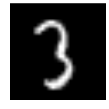 The above image is represented as numpy array, as seen below
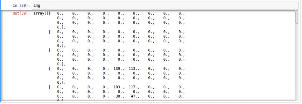 For easier data manipulation, let's store all our images as numpy arrays
temp = []
for img_name in train.filename:
image_path = os.path.join(data_dir, 'Train', 'Images', 'train', img_name)
img = imread(image_path, flatten=True)
img = img.astype('float32')
temp.append(img)
train_x = np.stack(temp)
temp = []
for img_name in test.filename:
image_path = os.path.join(data_dir, 'Train', 'Images', 'test', img_name)
img = imread(image_path, flatten=True)
img = img.astype('float32')
temp.append(img)
test_x = np.stack(temp)
As this is a typical ML problem, to test the proper functioning of our model we create a validation set.
Let's take a split size of 70:30 for train set vs validation set
split_size = int(train_x.shape[0]*0.7)
train_x, val_x = train_x[:split_size], train_x[split_size:]
train_y, val_y = train.label.ix[:split_size], train.label.ix[split_size:]
Now we define some helper functions, which we use later on, in our programs
def dense_to_one_hot(labels_dense, num_classes=10):
"""Convert class labels from scalars to one-hot vectors"""
num_labels = labels_dense.shape[0]
index_offset = numpy.arange(num_labels) * num_classes
labels_one_hot = numpy.zeros((num_labels, num_classes))
labels_one_hot.flat[index_offset + labels_dense.ravel()] = 1
return labels_one_hot
def preproc(unclean_batch_x):
"""Convert values to range 0-1"""
temp_batch = unclean_batch_x / unclean_batch_x.max()
return temp_batch
def batch_creator(batch_size, dataset_length, dataset_name):
"""Create batch with random samples and return appropriate format"""
batch_mask = rng.choice(dataset_length, batch_size)
batch_x = eval(dataset_name + '_x')[[batch_mask]].reshape(-1, 784)
batch_x = preproc(batch_x)
if dataset_name == 'train':
batch_y = eval(dataset_name).ix[batch_mask, 'label'].values
batch_y = dense_to_one_hot(batch_y)
return batch_x, batch_y
Now comes the main part! Let us define our neural network architecture.
We define a neural network with 3 layers; input, hidden and output.
The number of neurons in input and output are fixed, as the input is our 28 x 28 image and the output is a 10 x 1 vector representing the class.
We take 500 neurons in the hidden layer.
This number can vary according to your need.
We also assign values to remaining variables.
Read the article on fundamentals of neural network to know more in depth of how it works.
### set all variables
# number of neurons in each layer
input_num_units = 28*28
hidden_num_units = 500
output_num_units = 10
# define placeholders
x = tf.placeholder(tf.float32, [None, input_num_units])
y = tf.placeholder(tf.float32, [None, output_num_units])
# set remaining variables
epochs = 5
batch_size = 128
learning_rate = 0.01
### define weights and biases of the neural network (refer this article if you don't understand the terminologies)
weights = {
'hidden': tf.Variable(tf.random_normal([input_num_units, hidden_num_units], seed=seed)),
'output': tf.Variable(tf.random_normal([hidden_num_units, output_num_units], seed=seed))
}
biases = {
'hidden': tf.Variable(tf.random_normal([hidden_num_units], seed=seed)),
'output': tf.Variable(tf.random_normal([output_num_units], seed=seed))
}
Now create our neural networks computational graph
hidden_layer = tf.add(tf.matmul(x, weights['hidden']), biases['hidden'])
hidden_layer = tf.nn.relu(hidden_layer)
output_layer = tf.matmul(hidden_layer, weights['output']) + biases['output']
Also, we need to define cost of our neural network
cost = tf.reduce_mean(tf.nn.softmax_cross_entropy_with_logits(output_layer, y))
And set the optimizer, i.e.
our backpropogation algorithm.
Here we use Adam, which is an efficient variant of Gradient Descent algorithm.
There are a number of other optimizers available in tensorflow (refer here)
optimizer = tf.train.AdamOptimizer(learning_rate=learning_rate).minimize(cost)
After defining our neural network architecture, let's initialize all the variables
init = tf.initialize_all_variables()
Now let us create a session, and run our neural network in the session.
We also validate our models accuracy on validation set that we created
with tf.Session() as sess:
# create initialized variables
sess.run(init)
### for each epoch, do:
### for each batch, do:
### create pre-processed batch
### run optimizer by feeding batch
### find cost and reiterate to minimize
for epoch in range(epochs):
avg_cost = 0
total_batch = int(train.shape[0]/batch_size)
for i in range(total_batch):
batch_x, batch_y = batch_creator(batch_size, train_x.shape[0], 'train')
_, c = sess.run([optimizer, cost], feed_dict = {x: batch_x, y: batch_y})
avg_cost += c / total_batch
print "Epoch:", (epoch+1), "cost =", "{:.5f}".format(avg_cost)
print "\nTraining complete!"
# find predictions on val set
pred_temp = tf.equal(tf.argmax(output_layer, 1), tf.argmax(y, 1))
accuracy = tf.reduce_mean(tf.cast(pred_temp, "float"))
print "Validation Accuracy:", accuracy.eval({x: val_x.reshape(-1, 784), y: dense_to_one_hot(val_y.values)})
predict = tf.argmax(output_layer, 1)
pred = predict.eval({x: test_x.reshape(-1, 784)})
This will be the output of the above code
Epoch: 1 cost = 8.93566
Epoch: 2 cost = 1.82103
Epoch: 3 cost = 0.98648
Epoch: 4 cost = 0.57141
Epoch: 5 cost = 0.44550
Training complete!
Validation Accuracy: 0.952823
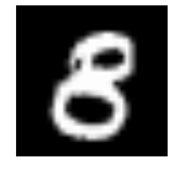
To test our model with our own eyes, let's visualize its predictions
img_name = rng.choice(test.filename)
filepath = os.path.join(data_dir, 'Train', 'Images', 'test', img_name)
img = imread(filepath, flatten=True)
test_index = int(img_name.split('.')[0]) - 49000
print "Prediction is: ", pred[test_index]
pylab.imshow(img, cmap='gray')
pylab.axis('off')
pylab.show()
Prediction is: 8
For easier data manipulation, let's store all our images as numpy arrays
temp = []
for img_name in train.filename:
image_path = os.path.join(data_dir, 'Train', 'Images', 'train', img_name)
img = imread(image_path, flatten=True)
img = img.astype('float32')
temp.append(img)
train_x = np.stack(temp)
temp = []
for img_name in test.filename:
image_path = os.path.join(data_dir, 'Train', 'Images', 'test', img_name)
img = imread(image_path, flatten=True)
img = img.astype('float32')
temp.append(img)
test_x = np.stack(temp)
As this is a typical ML problem, to test the proper functioning of our model we create a validation set.
Let's take a split size of 70:30 for train set vs validation set
split_size = int(train_x.shape[0]*0.7)
train_x, val_x = train_x[:split_size], train_x[split_size:]
train_y, val_y = train.label.ix[:split_size], train.label.ix[split_size:]
Now we define some helper functions, which we use later on, in our programs
def dense_to_one_hot(labels_dense, num_classes=10):
"""Convert class labels from scalars to one-hot vectors"""
num_labels = labels_dense.shape[0]
index_offset = numpy.arange(num_labels) * num_classes
labels_one_hot = numpy.zeros((num_labels, num_classes))
labels_one_hot.flat[index_offset + labels_dense.ravel()] = 1
return labels_one_hot
def preproc(unclean_batch_x):
"""Convert values to range 0-1"""
temp_batch = unclean_batch_x / unclean_batch_x.max()
return temp_batch
def batch_creator(batch_size, dataset_length, dataset_name):
"""Create batch with random samples and return appropriate format"""
batch_mask = rng.choice(dataset_length, batch_size)
batch_x = eval(dataset_name + '_x')[[batch_mask]].reshape(-1, 784)
batch_x = preproc(batch_x)
if dataset_name == 'train':
batch_y = eval(dataset_name).ix[batch_mask, 'label'].values
batch_y = dense_to_one_hot(batch_y)
return batch_x, batch_y
Now comes the main part! Let us define our neural network architecture.
We define a neural network with 3 layers; input, hidden and output.
The number of neurons in input and output are fixed, as the input is our 28 x 28 image and the output is a 10 x 1 vector representing the class.
We take 500 neurons in the hidden layer.
This number can vary according to your need.
We also assign values to remaining variables.
Read the article on fundamentals of neural network to know more in depth of how it works.
### set all variables
# number of neurons in each layer
input_num_units = 28*28
hidden_num_units = 500
output_num_units = 10
# define placeholders
x = tf.placeholder(tf.float32, [None, input_num_units])
y = tf.placeholder(tf.float32, [None, output_num_units])
# set remaining variables
epochs = 5
batch_size = 128
learning_rate = 0.01
### define weights and biases of the neural network (refer this article if you don't understand the terminologies)
weights = {
'hidden': tf.Variable(tf.random_normal([input_num_units, hidden_num_units], seed=seed)),
'output': tf.Variable(tf.random_normal([hidden_num_units, output_num_units], seed=seed))
}
biases = {
'hidden': tf.Variable(tf.random_normal([hidden_num_units], seed=seed)),
'output': tf.Variable(tf.random_normal([output_num_units], seed=seed))
}
Now create our neural networks computational graph
hidden_layer = tf.add(tf.matmul(x, weights['hidden']), biases['hidden'])
hidden_layer = tf.nn.relu(hidden_layer)
output_layer = tf.matmul(hidden_layer, weights['output']) + biases['output']
Also, we need to define cost of our neural network
cost = tf.reduce_mean(tf.nn.softmax_cross_entropy_with_logits(output_layer, y))
And set the optimizer, i.e.
our backpropogation algorithm.
Here we use Adam, which is an efficient variant of Gradient Descent algorithm.
There are a number of other optimizers available in tensorflow (refer here)
optimizer = tf.train.AdamOptimizer(learning_rate=learning_rate).minimize(cost)
After defining our neural network architecture, let's initialize all the variables
init = tf.initialize_all_variables()
Now let us create a session, and run our neural network in the session.
We also validate our models accuracy on validation set that we created
with tf.Session() as sess:
# create initialized variables
sess.run(init)
### for each epoch, do:
### for each batch, do:
### create pre-processed batch
### run optimizer by feeding batch
### find cost and reiterate to minimize
for epoch in range(epochs):
avg_cost = 0
total_batch = int(train.shape[0]/batch_size)
for i in range(total_batch):
batch_x, batch_y = batch_creator(batch_size, train_x.shape[0], 'train')
_, c = sess.run([optimizer, cost], feed_dict = {x: batch_x, y: batch_y})
avg_cost += c / total_batch
print "Epoch:", (epoch+1), "cost =", "{:.5f}".format(avg_cost)
print "\nTraining complete!"
# find predictions on val set
pred_temp = tf.equal(tf.argmax(output_layer, 1), tf.argmax(y, 1))
accuracy = tf.reduce_mean(tf.cast(pred_temp, "float"))
print "Validation Accuracy:", accuracy.eval({x: val_x.reshape(-1, 784), y: dense_to_one_hot(val_y.values)})
predict = tf.argmax(output_layer, 1)
pred = predict.eval({x: test_x.reshape(-1, 784)})
This will be the output of the above code
Epoch: 1 cost = 8.93566
Epoch: 2 cost = 1.82103
Epoch: 3 cost = 0.98648
Epoch: 4 cost = 0.57141
Epoch: 5 cost = 0.44550
Training complete!
Validation Accuracy: 0.952823
To test our model with our own eyes, let's visualize its predictions
img_name = rng.choice(test.filename)
filepath = os.path.join(data_dir, 'Train', 'Images', 'test', img_name)
img = imread(filepath, flatten=True)
test_index = int(img_name.split('.')[0]) - 49000
print "Prediction is: ", pred[test_index]
pylab.imshow(img, cmap='gray')
pylab.axis('off')
pylab.show()
Prediction is: 8
 We see that our model performance is pretty good! Now let's create a submission
sample_submission.filename = test.filename
sample_submission.label = pred
sample_submission.to_csv(os.path.join(sub_dir, 'sub01.csv'), index=False)
And done! We just created our own trained neural network!
We see that our model performance is pretty good! Now let's create a submission
sample_submission.filename = test.filename
sample_submission.label = pred
sample_submission.to_csv(os.path.join(sub_dir, 'sub01.csv'), index=False)
And done! We just created our own trained neural network!
Limitations of TensorFlow
Even though TensorFlow is powerful, it's still a low level library. For example, it can be considered as a machine level language. But for most of the purpose, you need modularity and high level interface such as keras It's still in development, so much more awesomeness to come! It depends on your hardware specs, the more the merrier Still not an API for many languages. There are still many things yet to be included in TensorFlow, such as OpenCL support. Most of the above mentioned are in the sights of TensorFlow developers. They have made a roadmap for specifying how the library should be developed in the future.TensorFlow vs. Other Libraries
TensorFlow is built on similar principles as Theano and Torch of using mathematical computational graphs. But with the additional support of distributed computing, TensorFlow comes out to be better at solving complex problems. Also deployment of TensorFlow models is already supported which makes it easier to use for industrial purposes, giving a fight to commercial libraries such as Deeplearning4j, H2O and Turi. TensorFlow has APIs for Python, C++ and Matlab. There's also a recent surge for support for other languages such as Ruby and R. So, TensorFlow is trying to have a universal language support.Where to go from here?
So you saw how to build a simple neural network with TensorFlow. This code is meant for people to understand how to get started implementing TensorFlow, so take it with a pinch of salt. Remember that to solve more complex real life problems, you have to tweak the code a little bit. Many of the above functions can be abstracted to give a seamless end-to-end workflow. If you have worked with scikit-learn, you might know how a high level library abstracts "under the hood" implementations to give end-users a more easier interface. Although TensorFlow has most of the implementations already abstracted, high level libraries are emerging such as TF-slim and TFlearn.Useful Resources
TensorFlow official repository Rajat Monga (TensorFlow technical lead) "TensorFlow for everyone" video A curated list of dedicated resourcesDeep Learning Project with Keras
Keras Tutorial Overview
There is not a lot of code required. The steps to cover: Load Data. Define Keras Model. Compile Keras Model. Fit Keras Model. Evaluate Keras Model. Tie It All Together. Make Predictions This Keras tutorial has a few requirements: You have SciPy (including NumPy) installed and configured. You have Keras and a backend (Theano or TensorFlow) installed and configured. If you need help with your environment, see the tutorial: Create a new file called keras_first_network.py and type or copy-and-paste the code into the file as you go.Load Data
We will use the NumPy library to load our dataset and we will use two classes from the Keras library to define our model.
# first neural network with keras tutorial
from numpy import loadtxt
from keras.models import Sequential
from keras.layers import Dense
We can now load our dataset.
In this Keras tutorial, we are going to use the Pima Indians onset of diabetes dataset.
This is a standard machine learning dataset from the UCI Machine Learning repository.
It describes patient medical record data for Pima Indians and whether they had an onset of diabetes within five years.
As such, it is a binary classification problem (onset of diabetes as 1 or not as 0).
All of the input variables that describe each patient are numerical.
This makes it easy to use directly with neural networks that expect numerical input and output values, and ideal for our first neural network in Keras.
The dataset is available from here:
Dataset CSV File (pima-indians-diabetes.csv)
Dataset Details
Download the dataset and place it in your local working directory, the same location as your python file.
Save it with the filename:
pima-indians-diabetes.csv
Take a look inside the file, you should see rows of data like the following:
6,148,72,35,0,33.6,0.627,50,1
1,85,66,29,0,26.6,0.351,31,0
8,183,64,0,0,23.3,0.672,32,1
1,89,66,23,94,28.1,0.167,21,0
0,137,40,35,168,43.1,2.288,33,1
We can now load the file as a matrix of numbers using the NumPy function loadtxt().
There are eight input variables and one output variable (the last column).
We will be learning a model to map rows of input variables (X) to an output variable (y), which we often summarize as y = f(X).
The variables can be summarized as follows:
Input Variables (X):
Number of times pregnant
Plasma glucose concentration a 2 hours in an oral glucose tolerance test
Diastolic blood pressure (mm Hg)
Triceps skin fold thickness (mm)
2-Hour serum insulin (mu U/ml)
Body mass index (weight in kg/(height in m)^2)
Diabetes pedigree function
Age (years)
Output Variables (y):
Class variable (0 or 1)
Once the CSV file is loaded into memory, we can split the columns of data into input and output variables.
The data will be stored in a 2D array where the first dimension is rows and the second dimension is columns, e.g. [rows, columns].
We can split the array into two arrays by selecting subsets of columns using the standard NumPy slice operator or “:” We can select the first 8 columns from index 0 to index 7 via the slice 0:8.
We can then select the output column (the 9th variable) via index 8.
...
# load the dataset
dataset = loadtxt('pima-indians-diabetes.csv', delimiter=',')
# split into input (X) and output (y) variables
X = dataset[:,0:8]
y = dataset[:,8]
We are now ready to define our neural network model.
Note, the dataset has 9 columns and the range 0:8 will select columns from 0 to 7, stopping before index 8.
If this is new to you, then you can learn more about array slicing and ranges in this post:
How to Index, Slice and Reshape NumPy Arrays for Machine Learning in Python
Define Keras Model
Models in Keras are defined as a sequence of layers. We create a Sequential model and add layers one at a time until we are happy with our network architecture. The first thing to get right is to ensure the input layer has the right number of input features. This can be specified when creating the first layer with the input_dim argument and setting it to 8 for the 8 input variables. How do we know the number of layers and their types? This is a very hard question. There are heuristics that we can use and often the best network structure is found through a process of trial and error experimentation (I explain more about this here). Generally, you need a network large enough to capture the structure of the problem. In this example, we will use a fully-connected network structure with three layers. Fully connected layers are defined using the Dense class. We can specify the number of neurons or nodes in the layer as the first argument, and specify the activation function using the activation argument. We will use the rectified linear unit activation function referred to as ReLU on the first two layers and the Sigmoid function in the output layer. It used to be the case that Sigmoid and Tanh activation functions were preferred for all layers. These days, better performance is achieved using the ReLU activation function. We use a sigmoid on the output layer to ensure our network output is between 0 and 1 and easy to map to either a probability of class 1 or snap to a hard classification of either class with a default threshold of 0.5. We can piece it all together by adding each layer: The model expects rows of data with 8 variables (the input_dim=8 argument) The first hidden layer has 12 nodes and uses the relu activation function. The second hidden layer has 8 nodes and uses the relu activation function. The output layer has one node and uses the sigmoid activation function. ... # define the keras model model = Sequential() model.add(Dense(12, input_dim=8, activation='relu')) model.add(Dense(8, activation='relu')) model.add(Dense(1, activation='sigmoid')) ... Note, the most confusing thing here is that the shape of the input to the model is defined as an argument on the first hidden layer. This means that the line of code that adds the first Dense layer is doing 2 things, defining the input or visible layer and the first hidden layer.Compile Keras Model
Now that the model is defined, we can compile it. Compiling the model uses the efficient numerical libraries under the covers (the so-called backend) such as Theano or TensorFlow. The backend automatically chooses the best way to represent the network for training and making predictions to run on your hardware, such as CPU or GPU or even distributed. When compiling, we must specify some additional properties required when training the network. Remember training a network means finding the best set of weights to map inputs to outputs in our dataset. We must specify the loss function to use to evaluate a set of weights, the optimizer is used to search through different weights for the network and any optional metrics we would like to collect and report during training. In this case, we will use cross entropy as the loss argument. This loss is for a binary classification problems and is defined in Keras as “binary_crossentropy“. You can learn more about choosing loss functions based on your problem here: How to Choose Loss Functions When Training Deep Learning Neural Networks We will define the optimizer as the efficient stochastic gradient descent algorithm “adam“. This is a popular version of gradient descent because it automatically tunes itself and gives good results in a wide range of problems. To learn more about the Adam version of stochastic gradient descent see the post: Gentle Introduction to the Adam Optimization Algorithm for Deep Learning Finally, because it is a classification problem, we will collect and report the classification accuracy, defined via the metrics argument. ... # compile the keras model model.compile(loss='binary_crossentropy', optimizer='adam', metrics=['accuracy']) ...Fit Keras Model
We have defined our model and compiled it ready for efficient computation. Now it is time to execute the model on some data. We can train or fit our model on our loaded data by calling the fit() function on the model. Training occurs over epochs and each epoch is split into batches. Epoch: One pass through all of the rows in the training dataset. Batch: One or more samples considered by the model within an epoch before weights are updated. One epoch is comprised of one or more batches, based on the chosen batch size and the model is fit for many epochs. For more on the difference between epochs and batches, see the post: What is the Difference Between a Batch and an Epoch in a Neural Network? The training process will run for a fixed number of iterations through the dataset called epochs, that we must specify using the epochs argument. We must also set the number of dataset rows that are considered before the model weights are updated within each epoch, called the batch size and set using the batch_size argument. For this problem, we will run for a small number of epochs (150) and use a relatively small batch size of 10. These configurations can be chosen experimentally by trial and error. We want to train the model enough so that it learns a good (or good enough) mapping of rows of input data to the output classification. The model will always have some error, but the amount of error will level out after some point for a given model configuration. This is called model convergence. ... # fit the keras model on the dataset model.fit(X, y, epochs=150, batch_size=10) ... This is where the work happens on your CPU or GPU. No GPU is required for this example, but if you’re interested in how to run large models on GPU hardware cheaply in the cloud, see this post: How to Setup Amazon AWS EC2 GPUs to Train Keras Deep Learning ModelsEvaluate Keras Model
We have trained our neural network on the entire dataset and we can evaluate the performance of the network on the same dataset. This will only give us an idea of how well we have modeled the dataset (e.g. train accuracy), but no idea of how well the algorithm might perform on new data. We have done this for simplicity, but ideally, you could separate your data into train and test datasets for training and evaluation of your model. You can evaluate your model on your training dataset using the evaluate() function on your model and pass it the same input and output used to train the model. This will generate a prediction for each input and output pair and collect scores, including the average loss and any metrics you have configured, such as accuracy. The evaluate() function will return a list with two values. The first will be the loss of the model on the dataset and the second will be the accuracy of the model on the dataset. We are only interested in reporting the accuracy, so we will ignore the loss value. ... # evaluate the keras model _, accuracy = model.evaluate(X, y) print('Accuracy: %.2f' % (accuracy*100))Tie It All Together
You have just seen how you can easily create your first neural network model in Keras. Let’s tie it all together into a complete code example. # first neural network with keras tutorial from numpy import loadtxt from keras.models import Sequential from keras.layers import Dense # load the dataset dataset = loadtxt('pima-indians-diabetes.csv', delimiter=',') # split into input (X) and output (y) variables X = dataset[:,0:8] y = dataset[:,8] # define the keras model model = Sequential() model.add(Dense(12, input_dim=8, activation='relu')) model.add(Dense(8, activation='relu')) model.add(Dense(1, activation='sigmoid')) # compile the keras model model.compile(loss='binary_crossentropy', optimizer='adam', metrics=['accuracy']) # fit the keras model on the dataset model.fit(X, y, epochs=150, batch_size=10) # evaluate the keras model _, accuracy = model.evaluate(X, y) print('Accuracy: %.2f' % (accuracy*100)) You can copy all of the code into your Python file and save it as “keras_first_network.py” in the same directory as your data file “pima-indians-diabetes.csv“. You can then run the Python file as a script from your command line (command prompt) as follows: python keras_first_network.py 1 python keras_first_network.py Running this example, you should see a message for each of the 150 epochs printing the loss and accuracy, followed by the final evaluation of the trained model on the training dataset. It takes about 10 seconds to execute on my workstation running on the CPU. Ideally, we would like the loss to go to zero and accuracy to go to 1.0 (e.g. 100%). This is not possible for any but the most trivial machine learning problems. Instead, we will always have some error in our model. The goal is to choose a model configuration and training configuration that achieve the lowest loss and highest accuracy possible for a given dataset. ... 768/768 [==============================] - 0s 63us/step - loss: 0.4817 - acc: 0.7708 Epoch 147/150 768/768 [==============================] - 0s 63us/step - loss: 0.4764 - acc: 0.7747 Epoch 148/150 768/768 [==============================] - 0s 63us/step - loss: 0.4737 - acc: 0.7682 Epoch 149/150 768/768 [==============================] - 0s 64us/step - loss: 0.4730 - acc: 0.7747 Epoch 150/150 768/768 [==============================] - 0s 63us/step - loss: 0.4754 - acc: 0.7799 768/768 [==============================] - 0s 38us/step Accuracy: 76.56 Note, if you try running this example in an IPython or Jupyter notebook you may get an error. The reason is the output progress bars during training. You can easily turn these off by setting verbose=0 in the call to the fit() and evaluate() functions, for example: ... # fit the keras model on the dataset without progress bars model.fit(X, y, epochs=150, batch_size=10, verbose=0) # evaluate the keras model _, accuracy = model.evaluate(X, y, verbose=0) ... Note: Your results may vary given the stochastic nature of the algorithm or evaluation procedure, or differences in numerical precision. Consider running the example a few times and compare the average outcome. What score did you get?Post your results in the comments below. Neural networks are a stochastic algorithm, meaning that the same algorithm on the same data can train a different model with different skill each time the code is run. This is a feature, not a bug. You can learn more about this in the post: Embrace Randomness in Machine Learning The variance in the performance of the model means that to get a reasonable approximation of how well your model is performing, you may need to fit it many times and calculate the average of the accuracy scores. For more on this approach to evaluating neural networks, see the post: How to Evaluate the Skill of Deep Learning Models For example, below are the accuracy scores from re-running the example 5 times: Accuracy: 75.00 Accuracy: 77.73 Accuracy: 77.60 Accuracy: 78.12 Accuracy: 76.17 We can see that all accuracy scores are around 77% and the average is 76.924%.
Make Predictions
The number one question I get asked is:After I train my model, how can I use it to make predictions on new data?Great question. We can adapt the above example and use it to generate predictions on the training dataset, pretending it is a new dataset we have not seen before. Making predictions is as easy as calling the predict() function on the model. We are using a sigmoid activation function on the output layer, so the predictions will be a probability in the range between 0 and 1. We can easily convert them into a crisp binary prediction for this classification task by rounding them. For example: ... # make probability predictions with the model predictions = model.predict(X) # round predictions rounded = [round(x[0]) for x in predictions] Alternately, we can call the predict_classes() function on the model to predict crisp classes directly, for example: ... # make class predictions with the model predictions = model.predict_classes(X) The complete example below makes predictions for each example in the dataset, then prints the input data, predicted class and expected class for the first 5 examples in the dataset. # first neural network with keras make predictions from numpy import loadtxt from keras.models import Sequential from keras.layers import Dense # load the dataset dataset = loadtxt('pima-indians-diabetes.csv', delimiter=',') # split into input (X) and output (y) variables X = dataset[:,0:8] y = dataset[:,8] # define the keras model model = Sequential() model.add(Dense(12, input_dim=8, activation='relu')) model.add(Dense(8, activation='relu')) model.add(Dense(1, activation='sigmoid')) # compile the keras model model.compile(loss='binary_crossentropy', optimizer='adam', metrics=['accuracy']) # fit the keras model on the dataset model.fit(X, y, epochs=150, batch_size=10, verbose=0) # make class predictions with the model predictions = model.predict_classes(X) # summarize the first 5 cases for i in range(5): print('%s => %d (expected %d)' % (X[i].tolist(), predictions[i], y[i])) Running the example does not show the progress bar as before as we have set the verbose argument to 0. After the model is fit, predictions are made for all examples in the dataset, and the input rows and predicted class value for the first 5 examples is printed and compared to the expected class value. We can see that most rows are correctly predicted. In fact, we would expect about 76.9% of the rows to be correctly predicted based on our estimated performance of the model in the previous section. [6.0, 148.0, 72.0, 35.0, 0.0, 33.6, 0.627, 50.0] => 0 (expected 1) [1.0, 85.0, 66.0, 29.0, 0.0, 26.6, 0.351, 31.0] => 0 (expected 0) [8.0, 183.0, 64.0, 0.0, 0.0, 23.3, 0.672, 32.0] => 1 (expected 1) [1.0, 89.0, 66.0, 23.0, 94.0, 28.1, 0.167, 21.0] => 0 (expected 0) [0.0, 137.0, 40.0, 35.0, 168.0, 43.1, 2.288, 33.0] => 1 (expected 1) If you would like to know more about how to make predictions with Keras models, see the post: How to Make Predictions with Keras
Keras Tutorial Summary
In this post, you discovered how to create your first neural network model using the powerful Keras Python library for deep learning. Specifically, you learned the six key steps in using Keras to create a neural network or deep learning model, step-by-step including: How to load data. How to define a neural network in Keras. How to compile a Keras model using the efficient numerical backend. How to train a model on data. How to evaluate a model on data. How to make predictions with the model. Do you have any questions about Keras or about this tutorial?Ask your question in the comments and I will do my best to answer.